Getting Started#
pyopenms_viz allows users to visualize mass spectrometry data with minimal effort, making it ideal for software developers who do not want to focus on plotting, bioinformaticians wanting to explore their data in a python setting or experimental scientists who want more control of their data.
This is accomplished by providing a plotting interface ontop of the already widely used pandas dataframe.
This tutorial demonstrates the basic usage of pyopenms_viz, a plotting interface built on top of pandas for generating mass spectrometry plots like spectra, chromatograms, and peak maps.
Tutorial Requirements:#
pyopenmsfor.mzMLdata loadingalphatimsfor.ddata loading
[1]:
!pip install pyopenms alphatims --quiet
!pip install pandas==2.1.4 --quiet # this version avoids warning messages with alphatims
[2]:
import pyopenms
pyopenms.__version__
[2]:
'3.3.0'
[3]:
import alphatims
alphatims.__version__
[3]:
'1.0.9'
[4]:
import pandas as pd
pd.__version__
[4]:
'2.1.4'
Overview#
pyopenms-viz is a plotting framework supporting multiple plot common mass spectrometry plot types including the Spectrum, Chromatogram, PeakMap and Mobilogram. Plotting is achieved by calling the plot() method on a pd.DataFrame object containing mass spectrometry data in long format. For more information on how to format your data into a pd.DataFrame please see Data Formatting
The plot() Method#
The only function required for users of pyopenms_viz is the plot() method. This method is called directly on a pandas dataframe storing mass spectrometry data in the long format. This means that each row represents a single peak.
Required Arguments#
x - The column name of the x-axis
y - The column name of the y-axis
z (only peakmaps) - The column name of the z-axis - represented as colour in the peakmaps
kind - The kind of plot, options include:
"spectrum"- mass-to-charge ratio vs intensity vertical line plot"chromatogram"- retention time vs intensity line plot"peakmap"- scatterplot with z axes represented by color"mobilogram"- ion mobility vs intensity line plot
Backend - The backend to plot. can be one of “ms_matplotlib”, “ms_plotly” or “ms_bokeh”
ms_matplotlib - Standard python plotting backend, good for generating publication quality static plots
ms_bokeh - Lightweight interactive plotting
ms_plotly - Feature rich interactive plotting, also supports 3D plots, good integration with streamlit
Note
Backend can also be set globally using
pd.options.plotting.backend = 'ms_bokeh'
Optional Arguments#
Plots are highly customizable with additional arguments passed to the plot() method. For a full list of supported. A few notable optional arguments are mentioned below.
by - Grouping of the data, functionality depends on the plot type.
Spectrum = colors peaks based on grouping
Chromatogram/Mobilogram = Draw a separate line trace for each grouping
PeakMap = Different markers (e.g. “+”, “.” ..) for peaks of different groups
show_plot (default = True) - If
True, the method returnsNoneand the plot output. IfFalsethe plot is not shown and the function returns the underlying figure/axes object (depending on backend)
For a full list of arguments please see Parameters
Plot a Spectrum#
The Spectrum is one of the most commonly used plots in mass spectrometry. It contains mass-to-charge ratio on the x-axis and intensity on the y-axis.
Downloading the Data#
In this example, we will use pyopenms to load the .mzML file into a pandas dataframe. Examples using different packages can be found here.
[5]:
from urllib.request import urlretrieve
gh = "https://raw.githubusercontent.com/OpenMS/pyopenms-docs/master"
urlretrieve(
gh + "/src/data/PrecursorPurity_input.mzML", "test.mzML"
)
urlretrieve(
gh + "/src/data/YIC(Carbamidomethyl)DNQDTISSK.mzML", "YIC(Carbamidomethyl)DNQDTISSK.mzML"
)
[5]:
('YIC(Carbamidomethyl)DNQDTISSK.mzML',
<http.client.HTTPMessage at 0x7f06e8588cb0>)
Reading the data into a pd.DataFrame with pyopenms#
[6]:
import pyopenms as oms
# Load the raw mass spectrometry data
exp = oms.MSExperiment()
oms.MzMLFile().load("YIC(Carbamidomethyl)DNQDTISSK.mzML", exp)
# Fetch the first spectrum
spectrum = oms.MSSpectrum(exp.getSpectrum(0))
# Export the spectrum to a pandas dataframe
spectrum_df = spectrum.get_df()
spectrum_df.head(5)
[6]:
| mz | intensity | ion_mobility | ion_mobility_unit | ms_level | precursor_mz | precursor_charge | native_id | sequence | ion_annotation | base peak m/z | base peak intensity | total ion current | lowest observed m/z | highest observed m/z | filter string | preset scan configuration | |
|---|---|---|---|---|---|---|---|---|---|---|---|---|---|---|---|---|---|
| 0 | 212.012451 | 6.041170 | NaN | <NONE> | 2 | 722.324707 | 2 | spectrum=2624 | 584 | 906 | 7561 | 212 | 1297 | ITMS + c NSI d w Full ms2 722.32@cid35.00 [185... | 2 | ||
| 1 | 217.039612 | 2.125546 | NaN | <NONE> | 2 | 722.324707 | 2 | spectrum=2624 | 584 | 906 | 7561 | 212 | 1297 | ITMS + c NSI d w Full ms2 722.32@cid35.00 [185... | 2 | ||
| 2 | 230.094986 | 6.776063 | NaN | <NONE> | 2 | 722.324707 | 2 | spectrum=2624 | 584 | 906 | 7561 | 212 | 1297 | ITMS + c NSI d w Full ms2 722.32@cid35.00 [185... | 2 | ||
| 3 | 231.250870 | 3.464486 | NaN | <NONE> | 2 | 722.324707 | 2 | spectrum=2624 | 584 | 906 | 7561 | 212 | 1297 | ITMS + c NSI d w Full ms2 722.32@cid35.00 [185... | 2 | ||
| 4 | 232.206757 | 2.642101 | NaN | <NONE> | 2 | 722.324707 | 2 | spectrum=2624 | 584 | 906 | 7561 | 212 | 1297 | ITMS + c NSI d w Full ms2 722.32@cid35.00 [185... | 2 |
Plot Using pyopenms_viz#
Now that we have the spectrum in a Pandas Dataframe, we can plot it using pyopenms_viz. Note that we must specify that the x-axis is the column labelled mz and the y-axis is the column labelled intensity. Furthermore, a backend must also be specified.
[7]:
spectrum_df.plot(kind='spectrum', x='mz', y='intensity', backend='ms_bokeh')
[7]:
As this plot is interactive we can zoom in using the bokeh toolbar and also hovering over the peaks will provide their annotations.
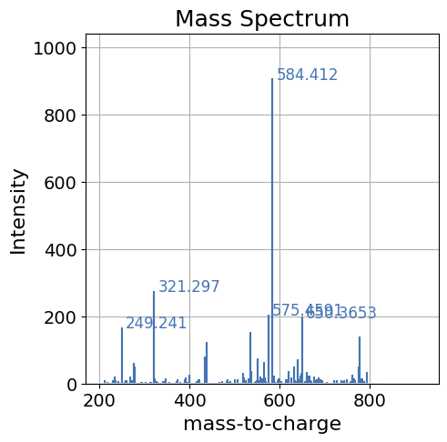
We can instead plot using matploltib by adjusting the backend.
[8]:
spectrum_df.plot(kind='spectrum', backend='ms_matplotlib', x='mz', y='intensity')
[8]:
<Axes: title={'center': 'Mass Spectrum'}, xlabel='mass-to-charge', ylabel='Intensity'>
Further Customization#
pyopenms_viz contains many options for plot customization. Some options are shown below. For a full list of options for customizing the spectrum please see the Spectrum Parameters
Base Customization Examples (Avalible for all graph types)#
Below are examples of customizations avaliable for all plot types. For a full list of customization options, please see Parameters
[9]:
base_kwargs = dict(kind='spectrum', x='mz', y='intensity', backend='ms_bokeh')
#spectrum_df.plot(grid=False, **base_kwargs) # no grid
#spectrum_df.plot(relative_intensity=False, **base_kwargs) # relative intensity
#spectrum_df.plot(xlabel='m/z', **base_kwargs) # change x label
Spectrum Specific Customization Examples#
These customizations below are specific to the spectrum plot
[10]:
base_kwargs = dict(kind='spectrum', x='mz', y='intensity', backend='ms_bokeh')
#spectrum_df.plot(bin_peaks=False, **base_kwargs) # no binning of peaks
spectrum_df.plot(annotate_top_n_peaks=0, **base_kwargs) # no peak annotation
[10]:
Even Further Customization#
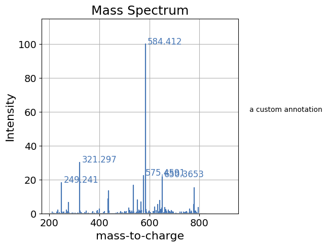
By default pyopenms_viz plot function returns nothing and just displays the plot. In the case where further customizations are required, by setting show_plot=False pyopenms_viz will return the underlying figure/axes object and further customizations can be performed with the underlying backend.
[11]:
import matplotlib.pyplot as plt
# Save plot in matplotlib axes object
ax = spectrum_df.plot(kind='spectrum', backend='ms_matplotlib', x='mz', y='intensity', relative_intensity=True, show_plot=False)
# add a custom text annotation
ax.text(1000, 60, "a custom annotation")
# display plot
plt.show()
Saving the Plot#
If you want to save the plot, you need to set show_plot=False, and then use the respective backend’s save method.
For matplotlib, you can use
plt.savefig(). For more information on saving matplotlib plots, see here.
p = spectrum_df.plot(
kind="spectrum",
x="mz",
y="intensity",
backend="ms_matplotlib",
show_plot=False
)
# Save a png file
plt.savefig('spectrum.png')
# Save an svg file
plt.savefig('spectrum.svg')
# Save a pdf file
plt.savefig('spectrum.pdf')
For bokeh, you can use
output_filemethod to save an html file of the iteractive plot. To save a static plot you can use the tool bar in the interactive plot to save the plot as a png. Or you can use theexport_pngmethod. However, this requires additional dependencies:pip install selenium geckodriver firefox. For more information on saving bokeh plots see here.
from bokeh.io import output_file
p = spectrum_df.plot(
kind="spectrum",
x="mz",
y="intensity",
backend="ms_bokeh",
show_plot=False
)
# Save a html file
output_file("spectrum.html")
For plotly, you can use
fig.write_html()method to save an html file of the interactive plot. To save a static plot you can use the tool bar in the interactive plot to save the plot as a png/svg/pdf. Or you can use thewrite_imagemethod. However, this requires additional dependencies:pip install -U kaleido. For more information on saving plotly plots see here.
p = spectrum_df.plot(
kind="spectrum",
x="mz",
y="intensity",
backend="ms_plotly",
show_plot=False
)
# Save a html file
p.write_html("spectrum.html")
Annotating A Spectrum#
If there is a peptide spectrum match, it is useful to annotate the spectrum with the fragments of the expected peptide so that one can manually evalute the match. Here, we demonstrate how to do this with pyopenms_viz and pyopenms
Create a mirror reference spectrum using pyopenms#
Using pyopenms we can create a theoretical spectrum on the peptide YIC(Carbamidomethyl)DNQDTISSK to compare with the experimental spectrum shown above. This is adapted from the pyopenms tutorial here
[12]:
# Generate theoretical spectrum
tsg = oms.TheoreticalSpectrumGenerator()
theo_spec = oms.MSSpectrum()
peptide = oms.AASequence.fromString("YIC(Carbamidomethyl)DNQDTISSK")
p = tsg.getParameters()
p.setValue("add_y_ions", "true")
p.setValue("add_b_ions", "true")
p.setValue("add_metainfo", "true")
tsg.setParameters(p)
tsg.getSpectrum(theo_spec, peptide, 1, 2)
theo_spec_df = theo_spec.get_df()
Plot the Spectrum and Mirror Spectrum#
To plot with pyopenms_viz, all that is required is the addtional reference_spectrum parameter which contains a pandas dataframe of the theoretical spectrum and to change mirror_spectrum to True
[13]:
spectrum_df.plot(kind='spectrum',
backend='ms_bokeh',
x='mz',
y='intensity',
annotate_top_n_peaks=0,
reference_spectrum=theo_spec_df,
title='Peptide YIC(Carbamidomethyl)DNQDTISSK',
title_font_size=12,
mirror_spectrum=True)
[13]:
Annotating the Experimental Spectrum#
We can annotate the experimental spectrum by aligning it to the theoretical spectrum and taking the labels of the fragment ions from the theoretical spectrum.
First we perform spectrum alignment using pyopenms
[14]:
alignment = []
spa = oms.SpectrumAlignment()
p = spa.getParameters()
# use 0.5 Da tolerance for m/z (Note: for high-resolution data we could also use ppm by setting the is_relative_tolerance value to true)
p.setValue("tolerance", 0.5)
p.setValue("is_relative_tolerance", "false")
spa.setParameters(p)
# align both spectra
spa.getSpectrumAlignment(alignment, theo_spec, spectrum)
Next we update the spectrum_df with the ion annotations
[15]:
for theo_spec_idx, exp_spec_idx in alignment:
spectrum_df.loc[exp_spec_idx, 'ion_annotation'] = theo_spec_df.loc[theo_spec_idx, 'ion_annotation']
Now that we have annotated the spectrum we can plot it. To include annotations in the plot pyopenms_viz expects a column name for the ion_annotation argument.
[16]:
spectrum_df.plot(kind='spectrum',
backend='ms_bokeh',
x='mz',
y='intensity',
annotate_top_n_peaks=3,
ion_annotation='ion_annotation',
title='Peptide YIC(Carbamidomethyl)DNQDTISSK',
title_font_size=12)
[16]:
By default when we set ion_annotation the y ions are colored in red and the b ions are colored in blue. Howevering over the peaks will now show the matched ion annotation
We can also combine the reference spectrum with the ion annotation in one plot.
[17]:
spectrum_df.plot(kind='spectrum',
backend='ms_bokeh',
x='mz',
y='intensity',
annotate_top_n_peaks=0,
ion_annotation='ion_annotation',
title='Peptide YIC(Carbamidomethyl)DNQDTISSK',
title_font_size=12,
legend_config=dict(show=False),
mirror_spectrum=True,
reference_spectrum=theo_spec_df)
[17]:
Plot a PeakMap#
A peakmap is a useful plot for generating an overview of the entire profile (MS1) data. In this representation all analytes can be visualized across time.
Download Data and Load Data#
Here, we are using a slice of 100 seconds of a metabolomics dataset which only contains MS1 information. In peakmap plots, it does not make sense to plot both MS1 and MS2 data in a single plot.
[18]:
gh = "https://raw.githubusercontent.com/OpenMS/pyopenms-docs/master"
urlretrieve(gh + "/src/data/FeatureFinderMetaboIdent_1_input.mzML", "test.mzML")
# open .mzML file using pyopenms
exp = oms.MSExperiment()
oms.MzMLFile().load("test.mzML", exp)
# convert pyopenms object to pandas dataframe
exp_df = exp.get_df(long=True)
exp_df
[18]:
| RT | mz | inty | ms_level | |
|---|---|---|---|---|
| 0 | 200.495300 | 250.117493 | 1078.637085 | 1 |
| 1 | 200.495300 | 250.118027 | 2352.115234 | 1 |
| 2 | 200.495300 | 250.118561 | 3718.094482 | 1 |
| 3 | 200.495300 | 250.119080 | 4042.395020 | 1 |
| 4 | 200.495300 | 250.119614 | 2848.561035 | 1 |
| ... | ... | ... | ... | ... |
| 117667 | 299.812897 | 274.114136 | 7654.166992 | 1 |
| 117668 | 299.812897 | 274.114746 | 10584.880859 | 1 |
| 117669 | 299.812897 | 274.115356 | 9032.423828 | 1 |
| 117670 | 299.812897 | 274.115967 | 5456.675293 | 1 |
| 117671 | 299.812897 | 274.116577 | 2176.139404 | 1 |
117672 rows × 4 columns
[19]:
exp_df.plot(kind='peakmap', backend='ms_bokeh', x='RT', y='mz', z='inty')
[19]:
PeakMap Specific Customization examples#
Below are some customizations that are specific to the "peakMap" plot. Note that some of these customizations, such as binning are also available for the "spectrum" plot however they are not avaliable for all plot types (e.g. "chromatogram"). For a full list of customizations please see the PeakMap Parameters.
Log-Scaling#
You can add the argument "z_log_scale = True" to log-scale the intensities (z-axis).
Useful when you want to enhance visualization of intensity variations or when you want to reduce dominant peak effects.
[20]:
#from bokeh.io import output_notebook
#output_notebook()
base_kwargs = dict(kind='peakmap', backend='ms_bokeh', x='RT', y='mz', z='inty')
exp_df.plot(z_log_scale=True, **base_kwargs)
[20]:
Adapting Bin Size in Peak Map Plots#
By default, the peak map uses binning to optimize visualization. You can adjust the binning level to balance between performance and detail.
Low binning (faster rendering, lower detail):
High binning (slower rendering, higher detail):
You can also remove binning of peaks adding the argument "bin_peaks = False", but can be slow on large datasets.
Below are examples demonstrating how to adjust bin size in peak map plots.
[21]:
# Example 1: Low binning (faster rendering, lower detail)
base_kwargs = dict(kind='peakmap', backend='ms_bokeh', x='RT', y='mz', z='inty')
exp_df.plot(num_x_bins=20, num_y_bins=20, **base_kwargs)
[21]:
[22]:
# Example 2: High binning (slower rendering, higher detail)
base_kwargs = dict(kind='peakmap', backend='ms_bokeh', x='RT', y='mz', z='inty')
exp_df.plot(num_x_bins=100, num_y_bins=100, **base_kwargs)
[22]:
[23]:
# Example 3: No bin peaks
base_kwargs = dict(kind='peakmap', backend='ms_bokeh', x='RT', y='mz', z='inty')
exp_df.plot(bin_peaks = False, **base_kwargs)
[23]:
PeakMap with Marginals#
One useful customization is to plot the peak map with marginal plots. The marginal plots sum the x and y axis respectively to provide a supplemental view of the data.
[24]:
base_kwargs = dict(kind='peakmap', backend='ms_bokeh', x='RT', y='mz', z='inty')
exp_df.plot(add_marginals=True, **base_kwargs)
/opt/hostedtoolcache/Python/3.12.10/x64/lib/python3.12/site-packages/pyopenms_viz/_bokeh/core.py:594: UserWarning:
You are attempting to set `plot.legend.orientation` on a plot that has zero legends added, this will have no effect.
Before legend properties can be set, you must add a Legend explicitly, or call a glyph method with a legend parameter set.
y_fig.legend.orientation = self.y_plot_config.legend_config.orientation
[24]:
Chromatogram Plot#
A chromatogram plot is useful for visualizing intensity across retention time. This can either be the total ion current across retention time or the ion curent from a specific region across m/z as used in targeted apporaches.
In this example, we will visualize the total ion current of the metabolomics dataset above. By default, pyopenms_viz does not manipulate the supplied
[25]:
exp_df.plot(kind='chromatogram', backend='ms_bokeh', x='RT', y='inty')
/opt/hostedtoolcache/Python/3.12.10/x64/lib/python3.12/site-packages/pyopenms_viz/_core.py:576: UserWarning: Duplicate data detected, data will not be aggregated which may lead to unexpected plots. To enable aggregation set `aggregate_duplicates=True`.
self._check_and_aggregate_duplicates()
[25]:
Note
By default pyopenms_viz does not manipulate the supplied dataframe meaning that there might be multiple points plotted at a single retention time value leading to unexpected plots. Peaks can be automatically summed up using aggregate_duplicates=True
[26]:
exp_df.plot(kind='chromatogram', backend='ms_bokeh', x='RT', y='inty', aggregate_duplicates=True)
[26]:
In this dataset different features are resolved nicely as indicated by nicely seperable peaks.
Chromatogram Specific Customizations#
For a full list of chromatogram specific customizations please see Chromatogram Parameters
Case Example: Inspecting a Peptide in DIA#
In this example, we will show how pyopenms_viz can be used to inspec a target peptide in Data Indepdent Acquisition. For this, we will be using a timsTOF dataset and show how pyopenms_viz integrates well with alphatims
Download the Data#
[27]:
import requests
import zipfile
import os
# Define the URL and file name
url = 'https://github.com/MannLabs/alphatims/releases/download/0.1.210317/20201207_tims03_Evo03_PS_SA_HeLa_200ng_EvoSep_prot_high_speed_21min_8cm_S1-C8_1_22474.d.zip'
file_name = '20201207_tims03_Evo03_PS_SA_HeLa_200ng_EvoSep_prot_high_speed_21min_8cm_S1-C8_1_22474.d.zip'
extract_dir = './' # Directory to extract the contents
# Download the file
response = requests.get(url)
with open(file_name, 'wb') as file:
file.write(response.content)
print(f'File {file_name} downloaded successfully!')
# Unzip the file
with zipfile.ZipFile(file_name, 'r') as zip_ref:
zip_ref.extractall(extract_dir)
print(f'File extracted to {extract_dir}!')
# Optionally, remove the zip file after extraction
os.remove(file_name)
print(f'Zip file {file_name} removed.')
File 20201207_tims03_Evo03_PS_SA_HeLa_200ng_EvoSep_prot_high_speed_21min_8cm_S1-C8_1_22474.d.zip downloaded successfully!
File extracted to ./!
Zip file 20201207_tims03_Evo03_PS_SA_HeLa_200ng_EvoSep_prot_high_speed_21min_8cm_S1-C8_1_22474.d.zip removed.
[28]:
import alphatims.bruker
bruker_dia_d_folder_name = "./20201207_tims03_Evo03_PS_SA_HeLa_200ng_EvoSep_prot_high_speed_21min_8cm_S1-C8_1_22474.d"
dia_data = alphatims.bruker.TimsTOF(bruker_dia_d_folder_name)
100%|██████████| 11868/11868 [00:08<00:00, 1322.59it/s]
Extracting Data for peptide#
Let’s modify the inspect_peptide method from alphatims/nbs /tutorial.ipynb to return a dataframe with extracted data for the target precursor and fragemnt ions.
[29]:
def inspect_peptide(
dia_data,
peptide,
ppm=50,
rt_tolerance=30, #seconds
mobility_tolerance=0.05, #1/k0
):
precursor_mz = peptide["mz"]
precursor_mobility = peptide["mobility"]
precursor_rt = peptide["rt"]
fragment_mzs = peptide["fragment_mzs"]
rt_slice = slice(
precursor_rt - rt_tolerance,
precursor_rt + rt_tolerance
)
im_slice = slice(
precursor_mobility - mobility_tolerance,
precursor_mobility + mobility_tolerance
)
precursor_mz_slice = slice(
precursor_mz / (1 + ppm / 10**6),
precursor_mz * (1 + ppm / 10**6)
)
precursor_indices = dia_data[
rt_slice,
im_slice,
0, #index 0 means that the quadrupole is not used
precursor_mz_slice,
"raw"
]
prec_df = dia_data.as_dataframe(precursor_indices)
prec_df['Annotation'] = 'prec'
# print(f"Info: Shape of prec - {prec_df.shape}")
all_dfs = []
all_dfs.append(prec_df)
for fragment_name, mz in fragment_mzs.items():
fragment_mz_slice = slice(
mz / (1 + ppm / 10**6),
mz * (1 + ppm / 10**6)
)
fragment_indices = dia_data[
rt_slice,
im_slice,
precursor_mz_slice,
fragment_mz_slice,
"raw"
]
frag_df = dia_data.as_dataframe(fragment_indices)
frag_df['Annotation'] = fragment_name
all_dfs.append(frag_df)
all_df = pd.concat(all_dfs, axis=0)
all_df['ms_level'] = all_df['Annotation'].apply(lambda x: 1 if x == 'prec' else 2)
return all_df
Let’s create a peptide dictionary with target coordinates for our target peptide
In order to extract a peptide, we need information on the peptide. For this example we will use peptide YNDTFWK below.
[30]:
peptide = {
"sequence": "YNDTFWK",
"mz": 487.22439,
"mobility": 0.81,
"rt": 9.011 * 60, #seconds
"charge": 2,
"fragment_mzs": {
"y7": 973.44145,
"y6": 810.37812,
"y5": 696.33520,
"y4": 581.30825,
"y3": 480.26057,
"y2": 333.19216,
"y1": 147.11285,
"b1": 164.07065,
"b2": 278.11358,
"b3": 393.14052,
"b4": 494.18820,
"b5": 641.25661,
"b6": 827.33592,
"b7": 955.43089,
}
}
[31]:
dia_df = inspect_peptide(dia_data, peptide, 50, 70, 0.1)
dia_df
[31]:
| raw_indices | frame_indices | scan_indices | precursor_indices | push_indices | tof_indices | rt_values | rt_values_min | mobility_values | quad_low_mz_values | quad_high_mz_values | mz_values | intensity_values | corrected_intensity_values | Annotation | ms_level | |
|---|---|---|---|---|---|---|---|---|---|---|---|---|---|---|---|---|
| 0 | 146798839 | 4438 | 694 | 0 | 4119158 | 152514 | 470.926503 | 7.848775 | 0.865903 | -1.0 | -1.0 | 487.228624 | 54 | 54 | prec | 1 |
| 1 | 146799536 | 4438 | 695 | 0 | 4119159 | 152515 | 470.926503 | 7.848775 | 0.864769 | -1.0 | -1.0 | 487.232119 | 68 | 68 | prec | 1 |
| 2 | 146802782 | 4438 | 700 | 0 | 4119164 | 152516 | 470.926503 | 7.848775 | 0.859099 | -1.0 | -1.0 | 487.235614 | 61 | 61 | prec | 1 |
| 3 | 146809110 | 4438 | 711 | 0 | 4119175 | 152519 | 470.926503 | 7.848775 | 0.846621 | -1.0 | -1.0 | 487.246098 | 144 | 144 | prec | 1 |
| 4 | 146809639 | 4438 | 712 | 0 | 4119176 | 152519 | 470.926503 | 7.848775 | 0.845486 | -1.0 | -1.0 | 487.246098 | 94 | 94 | prec | 1 |
| ... | ... | ... | ... | ... | ... | ... | ... | ... | ... | ... | ... | ... | ... | ... | ... | ... |
| 151 | 255542671 | 5684 | 671 | 4 | 5275423 | 264156 | 602.997099 | 10.049952 | 0.891960 | 475.0 | 500.0 | 955.470987 | 145 | 145 | b7 | 2 |
| 152 | 257300501 | 5702 | 746 | 4 | 5292202 | 264157 | 604.905047 | 10.081751 | 0.806864 | 475.0 | 500.0 | 955.475880 | 158 | 158 | b7 | 2 |
| 153 | 260842198 | 5738 | 715 | 4 | 5325579 | 264145 | 608.719248 | 10.145321 | 0.842081 | 475.0 | 500.0 | 955.417157 | 79 | 79 | b7 | 2 |
| 154 | 261754335 | 5747 | 749 | 4 | 5333965 | 264155 | 609.673048 | 10.161217 | 0.803453 | 475.0 | 500.0 | 955.466093 | 93 | 93 | b7 | 2 |
| 155 | 262643510 | 5756 | 730 | 4 | 5342298 | 264152 | 610.627758 | 10.177129 | 0.825048 | 475.0 | 500.0 | 955.451412 | 152 | 152 | b7 | 2 |
19375 rows × 16 columns
Globally Set Plotting Backend#
Let’s globally set the plotting backend so it does not have to be specified in each function call.
[32]:
pd.options.plotting.backend = 'ms_bokeh'
Chromatogram Plotting#
Let’s plot an extracted ion chromatgram, but before we do that, let’s preprocess the data and integrate the intensity values across ion mobility dimension to get an integrated extracted ion chromatogram per precursor and fragment ions.
If we plot the dia_df chromatograms at baseline, we will have multiple points per RT point (due to multiple points across ion mobility). To address this we can use the aggregate_duplicates=True argument. Furthermore, setting by='Annotation tells pyopenms_viz to plot each annotation as a seperate chromatogram.
[33]:
dia_df.plot(x='rt_values',
y='intensity_values',
kind='chromatogram',
by='Annotation', # each annotation as seperate chromatogram
aggregate_duplicates=True,
width=700,
legend_config=dict(title='Annotation'),
title="Extracted Chromatogram for YNDTFWK_2",
title_font_size=14)
[33]:
Based on the plot above, it looks like this peptide precursor elutes from 594.40 to 605 seconds. We can draw these boundaries on the chromatogram by specifiying the annotation_data dataframe. We can also extract across retention time to better see the feature.
[34]:
annotation_data = pd.DataFrame(dict(leftWidth=[594.40], rightWidth=[605]))
# filter df across rt
dia_df_small = dia_df[dia_df['rt_values'].between(500, 700)]
dia_df_small.plot(x='rt_values',
y='intensity_values',
kind='chromatogram',
by='Annotation', # each annotation as seperate chromatogram
aggregate_duplicates=True,
annotation_data=annotation_data,
width=700,
height=500,
legend_config = dict(title='Annotation'),
title="Extracted Chromatogram for YNDTFWK_2",
title_font_size=14)
[34]:
Grouping is not only limited to Annnotation we can change the by parameter to ms_level to get the total ion chromatograms for MS1 and MS2 levels respectively.
[35]:
annotation_data = pd.DataFrame(dict(leftWidth=[594.40], rightWidth=[605]))
# filter df across rt
dia_df_small = dia_df[dia_df['rt_values'].between(500, 700)]
dia_df_small.plot(x='rt_values',
y='intensity_values',
kind='chromatogram',
by='ms_level', # each ms_level as a seperate chromatogram
aggregate_duplicates=True,
annotation_data=annotation_data,
width=700,
height=500,
legend_config = dict(title='Annotation'),
title="Extracted Chromatogram for YNDTFWK_2",
title_font_size=14)
[35]:
Mobilogram Plotting#
We can also plot the extracted ion mobilogram as shown below
[36]:
group_cols=['ms_level', 'Annotation', 'mobility_values']
integrate_col = 'intensity_values'
dia_xim_df = dia_df.apply(
lambda x: x.fillna(0) if x.dtype.kind in "biufc" else x.fillna(".")
) \
.groupby(group_cols)[integrate_col] \
.sum() \
.reset_index()
[37]:
dia_df.plot(x='mobility_values',
y='intensity_values',
kind='mobilogram',
by='Annotation',
title = f"Extracted Spectrum for YNDTFWK_2",
height=500, width=700,
grid=False, # Remove the grid
aggregate_duplicates=True
)
[37]:
Spectrum Plotting#
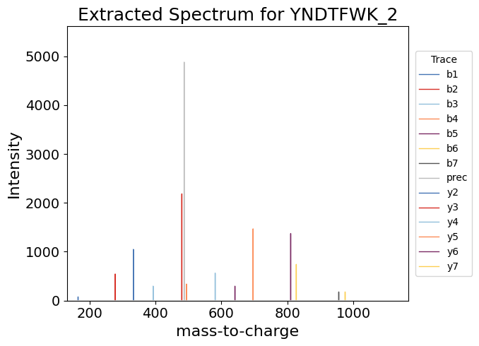
Let’s take a look at the extracted ion spectrum data. Since we have annotation labels for the extracted spectrum, we can add these to the plot as shown below. Here we will use the "ms_matplotlib" backend to generate a static plot.
[38]:
dia_df.plot(x="mz_values",
y="intensity_values",
kind="spectrum",
by="Annotation",
title = f"Extracted Spectrum for YNDTFWK_2",
backend='ms_matplotlib',
aggregate_duplicates=True,
height=500, width=700,
annotate_top_n_peaks=0,
grid=False, # Remove the grid
legend_config = dict(title='Trace', bbox_to_anchor=(1.2,0.5)))
[38]:
<Axes: title={'center': 'Extracted Spectrum for YNDTFWK_2'}, xlabel='mass-to-charge', ylabel='Intensity'>
2D Peak Map Plotting#
An alternative usage to the peakmap plot is to plot retetion time vs ion mobility for a single mass trace. This usage is demonstrated below. Let’s see what the retention time and ion mobility peak map looks like for the mass range of the precursor ion across all MS1 spectra.
[39]:
dia_df_prec = dia_df[dia_df['Annotation'] == 'prec']
[40]:
dia_df_prec.plot(x="rt_values",
y="mobility_values",
z="intensity_values",
kind="peakmap",
xlabel="Retention Time [sec]",
ylabel="Ion Mobility",
height=600,
width=700,
grid=False)
/opt/hostedtoolcache/Python/3.12.10/x64/lib/python3.12/site-packages/pyopenms_viz/_core.py:1133: UserWarning: Duplicate data detected, data will not be aggregated which may lead to unexpected plots. To enable aggregation set `aggregate_duplicates=True`.
self._check_and_aggregate_duplicates()
[40]:
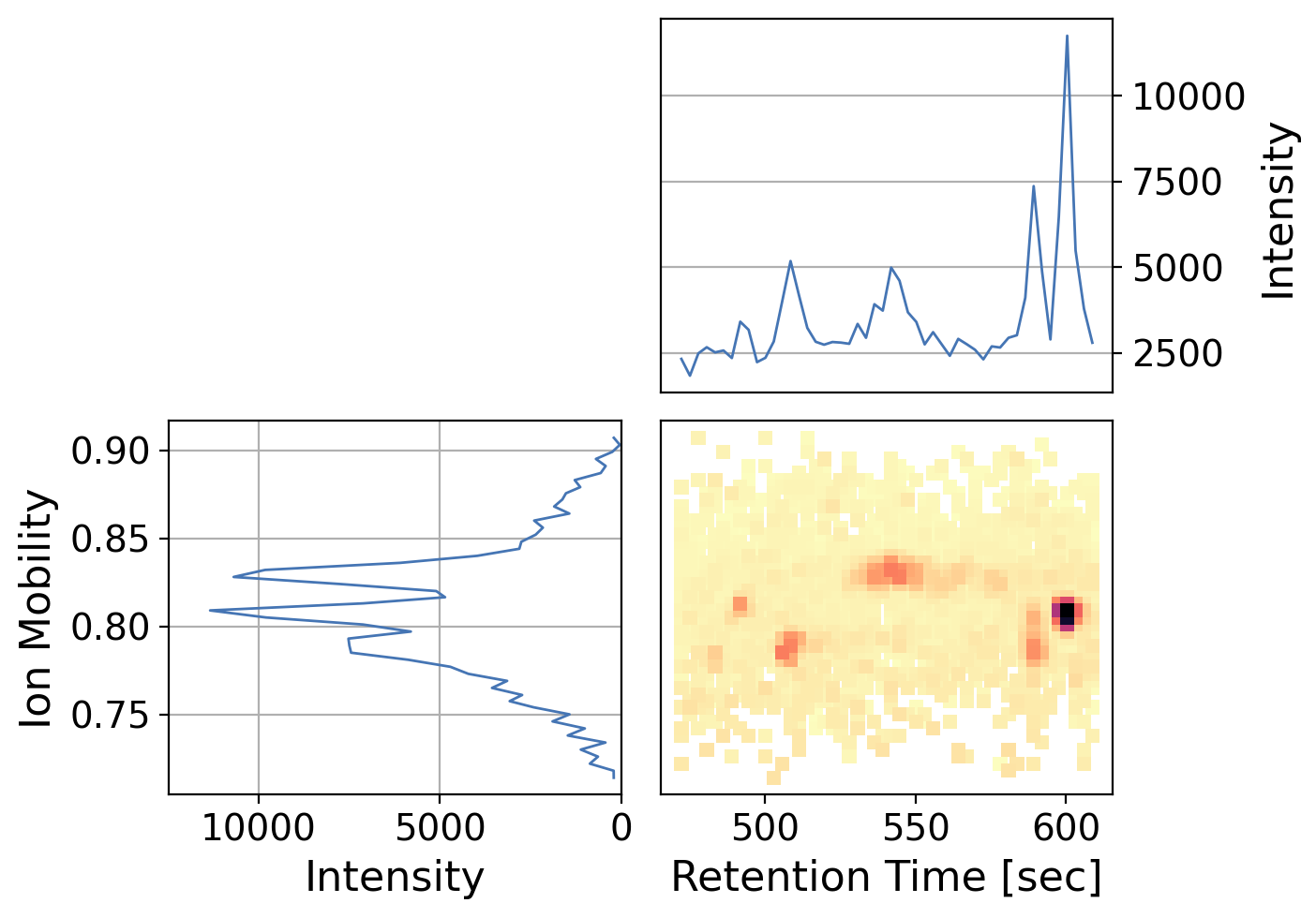
As expected, we see an intense signal with a retention time ~600 consistent with the chromatogram above and ion mobility of ~0.81.
Since intensity can be difficult to gauge only by color, we can also add marginal plots which sums up the x and y-axis respectively
[41]:
dia_df_prec.plot(x="rt_values",
y="mobility_values",
z="intensity_values",
kind="peakmap",
xlabel="Retention Time [sec]",
ylabel="Ion Mobility",
add_marginals=True,
width=700,
backend='ms_matplotlib',
y_kind='chromatogram', # specify on x marginal axis to plot as a chromatogram rather than a spectrum
x_kind='chromatogram', # specify on x marginal axis to plot as a chromatogram rather than a spectrum
grid=False)
/opt/hostedtoolcache/Python/3.12.10/x64/lib/python3.12/site-packages/pyopenms_viz/_core.py:1133: UserWarning: Duplicate data detected, data will not be aggregated which may lead to unexpected plots. To enable aggregation set `aggregate_duplicates=True`.
self._check_and_aggregate_duplicates()
[41]:

